5. Basic useage examples
In the following, usage of pycombina for solving binary approximation problems is exemplified.
5.1. Combinatorial integral approximation
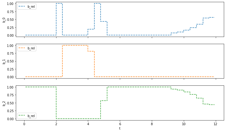
A binary approximation problem for a sample data set shall be solved using combinatorial integral approximation. The setup includes n_c = 3 mutually exclusive binary controls with each n_b = 149 values.
The first column of the file sample_data.csv contains the time points, the other columns contain the relaxed binary values.
[1]:
import numpy as np

data = np.loadtxt("sample_data_1.csv", skiprows = 1)

t = data[:,0]
b_rel = data[:-1,1:]
In the following, the data set is visualized.
[2]:
import matplotlib.pyplot as plt
%matplotlib inline

f, (ax1, ax2, ax3) = plt.subplots(3, sharex = True, figsize = (12,7))
ax1.step(t[:-1], b_rel[:,0], label = "b_rel", color = "C0", linestyle="dashed", where = "post")
ax1.set_ylabel("b_0")
ax1.legend(loc = "upper left")
ax2.step(t[:-1], b_rel[:,1], label = "b_rel",  color = "C1", linestyle="dashed", where = "post")
ax2.set_ylabel("b_1")
ax2.legend(loc = "upper left")
ax3.step(t[:-1], b_rel[:,2], label = "b_rel",  color = "C2", linestyle="dashed", where = "post")
ax3.set_ylabel("b_2")
ax3.legend(loc = "lower left")
ax3.set_xlabel("t")
plt.show()
First, we instantiate an object of the class pycombina.BinApprox to formulate the binary approximation problem, and check the problem dimensions.
[3]:
from pycombina import BinApprox

binapprox = BinApprox(t, b_rel)

assert(binapprox.n_c == 3)
assert(binapprox.n_t == t.size-1)
From the data shown above, it seems reasonable to set a maximum switching constraint for the controls.
[4]:
binapprox.set_n_max_switches(n_max_switches = [5, 2, 3])
For solution of the problem, we choose combinatorial integral approximation using the Branch-and-Bound method in pycombina.CombinaBnB.
[5]:
from pycombina import CombinaBnB

combina = CombinaBnB(binapprox)
combina.solve()
Running Branch and Bound ...

    Iteration   Upper bound    Branches     Runtime (s)
 U         62   6.146028e+00          116   4.380000e-04
 U         64   6.066028e+00          116   1.169000e-03
 U         66   5.986028e+00          116   1.192000e-03
 U         68   5.906028e+00          116   1.213000e-03
 U         70   5.826028e+00          116   1.233000e-03
 U         72   5.746028e+00          116   1.250000e-03
 U         74   5.666028e+00          116   1.268000e-03
 U         76   5.586028e+00          116   1.285000e-03
 U         78   5.506028e+00          116   1.301000e-03
 U         80   5.426028e+00          116   1.321000e-03
    Iteration   Upper bound    Branches     Runtime (s)
 U         82   5.346028e+00          116   1.339000e-03
 U         84   5.266028e+00          116   1.366000e-03
 U         86   5.186028e+00          116   1.384000e-03
 U         88   5.106028e+00          116   1.401000e-03
 U         90   5.026028e+00          116   1.418000e-03
 U         92   4.946028e+00          116   1.435000e-03
 U         94   4.866028e+00          116   1.452000e-03
 U         96   4.786028e+00          116   1.468000e-03
 U         98   4.706028e+00          116   1.487000e-03
 U        100   4.626028e+00          116   1.504000e-03
    Iteration   Upper bound    Branches     Runtime (s)
 U        102   4.546028e+00          116   1.520000e-03
 U        104   4.466028e+00          116   1.545000e-03
 U        106   4.386028e+00          116   1.726000e-03
 U        108   4.306028e+00          116   1.758000e-03
 U        110   4.226028e+00          116   1.786000e-03
 U        112   4.146028e+00          116   1.803000e-03
 U        114   4.066028e+00          116   1.821000e-03
 U        116   3.986028e+00          116   1.838000e-03
 U        118   3.906028e+00          116   1.855000e-03
 U        120   3.826028e+00          116   1.873000e-03
    Iteration   Upper bound    Branches     Runtime (s)
 U        122   3.746028e+00          116   1.890000e-03
 U        124   3.666028e+00          116   1.924000e-03
 U        126   3.586028e+00          116   1.942000e-03
 U        128   3.506028e+00          116   1.959000e-03
 U        130   3.426028e+00          116   1.976000e-03
 U        132   3.346028e+00          116   1.993000e-03
 U        134   3.266028e+00          116   2.009000e-03
 U        136   3.186028e+00          116   2.027000e-03
 U        138   3.106028e+00          116   2.044000e-03
 U        140   3.026028e+00          116   2.063000e-03
    Iteration   Upper bound    Branches     Runtime (s)
 U        142   2.946028e+00          116   2.080000e-03
 U        144   2.866028e+00          116   2.108000e-03
 U        146   2.786028e+00          116   2.125000e-03
 U        148   2.706028e+00          116   2.142000e-03
 U        150   2.626028e+00          116   2.161000e-03
 U        152   2.546028e+00          116   2.179000e-03
 U        154   2.466028e+00          116   2.198000e-03
 U        156   2.386028e+00          116   2.217000e-03
 U        158   2.306028e+00          116   2.234000e-03
 U        160   2.226028e+00          116   2.251000e-03
    Iteration   Upper bound    Branches     Runtime (s)
 U        162   2.146028e+00          116   2.267000e-03
 U        164   2.066028e+00          116   2.293000e-03
 U        166   1.986028e+00          116   2.309000e-03
 U        168   1.906028e+00          116   2.326000e-03
 U        170   1.826028e+00          116   2.342000e-03
 U        172   1.746028e+00          116   2.359000e-03
 U        174   1.666028e+00          116   2.385000e-03
 U        176   1.586028e+00          116   2.403000e-03
 U        178   1.506028e+00          116   2.419000e-03
 U        180   1.426028e+00          116   2.445000e-03
    Iteration   Upper bound    Branches     Runtime (s)
 U        182   1.346028e+00          116   2.483000e-03
 U        184   1.266028e+00          116   2.511000e-03
 U        186   1.186028e+00          116   2.528000e-03
 U        188   1.106028e+00          116   2.554000e-03
 U        190   1.026028e+00          116   2.571000e-03
 U        192   9.460280e-01          116   2.587000e-03
 U        194   8.660280e-01          116   2.604000e-03
 U        196   7.860280e-01          116   2.620000e-03
 U        198   7.060280e-01          116   2.636000e-03
 U        200   6.260280e-01          116   2.652000e-03
    Iteration   Upper bound    Branches     Runtime (s)
 U        202   5.460280e-01          116   2.668000e-03
 U        204   4.660280e-01          116   2.696000e-03
 U        206   3.860280e-01          116   2.722000e-03
 U        208   3.170696e-01          116   2.748000e-03
 U        285   3.060280e-01          116   2.889000e-03
 U        287   2.929646e-01          115   2.938000e-03
 U        364   2.409122e-01          116   3.066000e-03
 U        442   2.260280e-01          116   3.198000e-03
 U        444   2.168072e-01          115   3.251000e-03

    Optimal solution found

    Best solution:    2.168072e-01
    Total iterations:        22463
    Total runtime:    3.902900e-02 s
The solution times shown above have been achieved on an Intel Core i5-4570 3.20 GHz CPU.
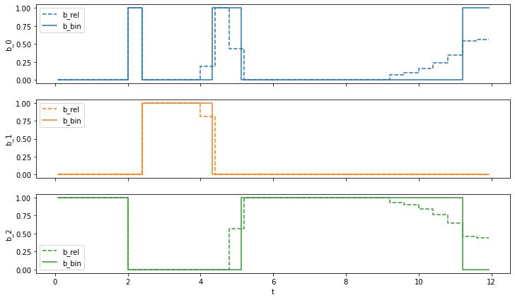
In the following, we can retrieve and inspect the obtained binary solution and the corresponding objective value.
[6]:
eta = binapprox.eta
b_bin = binapprox.b_bin

print("Objective value:", eta)
Objective value: 0.2168071999999996
[7]:
f, (ax1, ax2, ax3) = plt.subplots(3, sharex = True, figsize = (12,7))
ax1.step(t[:-1], b_rel[:,0], label = "b_rel", color = "C0", linestyle="dashed", where = "post")
ax1.step(t[:-1], b_bin[0,:], label = "b_bin", color = "C0", where = "post")
ax1.legend(loc = "upper left")
ax1.set_ylabel("b_0")
ax2.step(t[:-1], b_rel[:,1], label = "b_rel", color = "C1", linestyle="dashed", where = "post")
ax2.step(t[:-1], b_bin[1,:], label = "b_bin", color = "C1", where = "post")
ax2.legend(loc = "upper left")
ax2.set_ylabel("b_1")
ax3.step(t[:-1], b_rel[:,2], label = "b_rel", color = "C2", linestyle="dashed", where = "post")
ax3.step(t[:-1], b_bin[2,:], label = "b_bin", color = "C2", where = "post")
ax3.legend(loc = "lower left")
ax3.set_ylabel("b_2")
ax3.set_xlabel("t")
plt.show()
5.2. Sum up rounding
… tbd